How To Highlight Smallest Number In Excel Row

06 Sep, 2021

Finding the lowest or highest value in an Excel row or column is simple using. In this case the rank simply comes from column E.

How To Highlight Cells With Duplicate Values In A Range Excel Indian History Facts History Facts

Let me know in the commentsWant to see more.

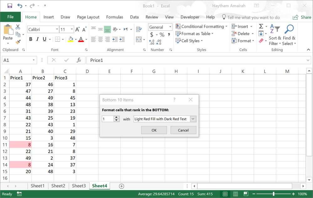
How to highlight smallest number in excel row. In our case the numbers are in B2B10 so we select it. How to highlight bottom values in Excel. Select Format only top or bottom ranked values as the rule type.

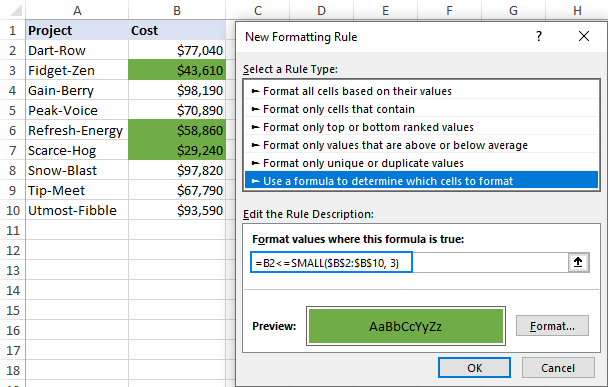
I want to highlight the smallest 3 numbers in this range. In the New Formatting Rule. Select a cell below or to the right of the numbers for which you want to find the smallest number.

Here is a quicker and more convenient array formula. Here select format only top or bottom ranked value In the drop-down select bottom. Highlight the minimum value in each row.

You can also add up the smallest 3 values with these array formulas as above steps. B2 MIN B2D2 Highlight Highest Value in Each Column. Lowest value to return.

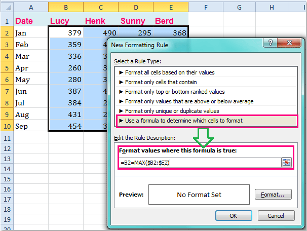
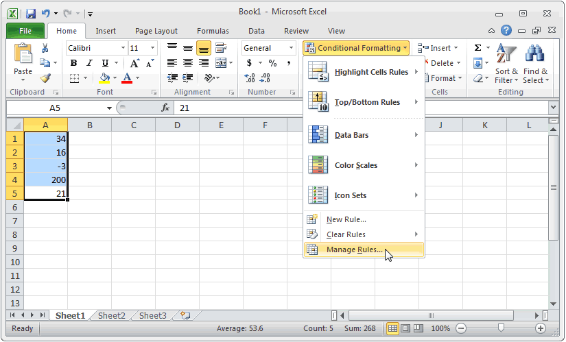
Select the range in which you want to highlight bottom values. SMALL range1 smallest SMALL range2 2nd smallest SMALL range3 3rd smallest. Home Conditional Formatting New Rule Use a formula to determine which cells to format.

Mark knows he can use the SMALL function with the second argument calculated by using a COUNTIF to count the number of zeroes in the range. Mark is hoping to find the smallest non-zero value in a set of values. If the cells are not in a contiguous row or column.

The small function can retrieve the smallest values from data based on rank. To highlight the 3 smallest values that meet specific criteria you can use an array formula based on the AND and SMALL functions. How to highlight largest lowest value in each row or column.

If youd like to highlight. On the Home tab in the Editing group click the arrow next to AutoSum click Min calculates the smallest or Max calculates the largest and then press ENTER. Type the following formula where C is the last column A1MIN A1C1 click Format button and apply the.

SMALL IF formula in Excel To get the n-th lowest value that matches the criteria you specify you can use the following generic formula. Select the range that captures the data you want to sort. Go to Home.

Select the first cell in the first row eg. In the example shown the formula used for conditional formatting is. AND B5 E5 C5.

In our example weve selected only the first bottom value. 1 Choose the type of cells that you want to use under the Look in section you can select the max or min value from value cells formula cells or. Like the videoHave another problem.

Then select Bottom in the first drop down and enter 1 in the final box. Highlight Lowest Value in Each Row If you want to highlight lowest value in each row in your table you just need to repeat the above steps just use the following formula instead of it. To highlight the smallest three value in excel follow these steps.

Office expert Susan Harkins teaches you two ways to highlight the lowest and highest values in an Excel row or column. HttpbitlyTAfDi6Did this help you out. Determines in case the smallest value exists in a particular column If ApplicationWorksheetFunctionCountIf rngCol vValue 0 Then Returns row number of the smallest value in the column which has the same lngRow ApplicationWorksheetFunctionMatch vValue rngCol 0.

Next we need to select what formatting to apply when this second condition is met. For example if he has the values 003068 he would want the value 3 the smallest non-zero value returned by a formula. After enter this formula remember to press Ctrl Shift Enter keys.

If you need to sum a different quantity of numbers just change the 20 to the desired number. 2 Specify the Minimum value or Maximum value that you want to select from the Go. Select data Home tab Sort Filter Custom Sort Options Select Sort left to right OK Select the Row by which to sort Select which to Sort on Select Smallest to Largest Order OK 1.

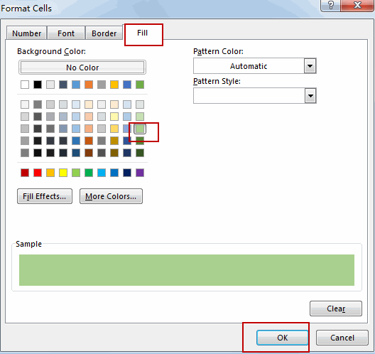
SMALL IF criteria_range criteria values n Where n is the 1 st 2 nd 3 rd etc. On the Home tab in the Styles group click Conditional formatting New Rule. To do this click on the Format button.

Pin By Elaine Weston On Career Stuff Microsoft Excel Excel Microsoft

Highlight Lowest In Row Episode 1206 Youtube

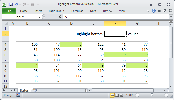
Excel Formula Highlight Bottom Values Exceljet

How To Highlight Largest Lowest Value In Each Row Or Column

How To Highlight The Highest And Lowest Value In Each Row Or Column In Excel Free Excel Tutorial

How To Highlight Largest Lowest Value In Each Row Or Column

Pin On Excel

Highlight The Minimum Value In Each Row Microsoft Tech Community

How To Highlight The Highest And Lowest Value In Each Row Or Column In Excel Free Excel Tutorial

How To Highlight Largest Lowest Value In Each Row Or Column

Automatically Highlight Rows With The Max Value In An Excel Data Table When You Are Looking At A Large List Of Numerical Data It S Usef Data Table Data Excel